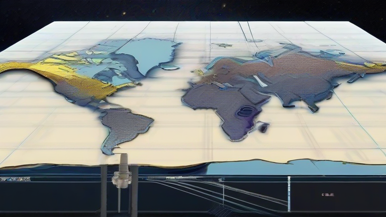
TL;DR: This guide explains how researchers and engineers will deploy the world’s first space-based quantum gravity sensor to create ultra-high-resolution maps of Earth’s subsurface mass. You’ll learn the step-by-step process—from payload calibration to orbital data stitching—that turns quantum interference into a 3D gravity map of our planet.
Step 1: Understand the Core Principle (Atom Interferometry)
Before touching hardware, grasp the physics. The sensor uses cold rubidium atoms cooled to near absolute zero. When these atoms are released in free-fall, a laser pulse splits each atom into a superposition of two quantum states—one taking a higher path, one a lower path. Gravity causes a phase shift between these paths when they recombine. That shift is directly proportional to local gravitational acceleration. Your mission is to measure that phase shift with picometer precision, not to build a “gravity meter” in the classical sense.
If you want to dig deeper, check out our guide on The Best Tech Gadgets Under $100: Real-World Tested Picks.
Step 2: Assemble the Payload in a Cleanroom (Class 100 or better)
Start with a vacuum chamber (10⁻¹¹ mbar). Inside, install a magneto-optical trap (MOT) to capture and cool rubidium-87 atoms. Add two counter-propagating laser systems: one for cooling (780 nm), one for Raman transitions (used to split/recombine atom waves). Mount the entire assembly on a vibration-isolation platform that cancels spacecraft micro-jitter to below 10⁻⁹ g/√Hz. Critical tip: use fiber-coupled lasers to avoid thermal drift—quantum sensors are hypersensitive to temperature gradients above 1 mK/s.
Step 3: Calibrate in a Ground-Based Drop Tower
Before launch, run a full vertical test. Drop the sensor in a 120-meter vacuum tower (e.g., ZARM in Bremen) to verify that the measured gravity gradient matches known local values. Record the phase shift vs. time curve. Calculate the scale factor (radians per mGal). Tip: perform at least 500 drops to average out seismic noise. Compare your results against a superconducting gravimeter—if deviation exceeds 0.1%, re-tune the laser power and Raman pulse duration.
Step 4: Launch and Achieve Stable Low-Earth Orbit (LEO)
Place the sensor on a small satellite (e.g., 150 kg class) in a sun-synchronous orbit at 400–500 km altitude. Inclination ~97° for global coverage. After deployment, wait 72 hours for outgassing and thermal equilibrium. Then, activate the internal cold-atom source—the system will automatically produce 10⁷ atoms per shot, every 1.5 seconds. Tip: keep the spacecraft’s attitude within ±0.01° of nadir (pointing straight down) to avoid Doppler shifts that corrupt the phase readout.
Step 5: Collect and Process Raw Quantum Data
For each measurement cycle, record three data streams: (1) the interference fringe pattern (intensity vs. laser phase), (2) the satellite’s precise position from GNSS, and (3) accelerometer data for non-gravitational forces (solar pressure, drag). Use a Kalman filter to fuse these. The output is a “gravity anomaly” value (in milliGals) at each point along the orbit. Tip: discard any shot where the fringe contrast drops below 70%—that indicates a cosmic-ray hit or laser power dropout.
Step 6: Stitch Data into a Global Gravity Map
After 30 days of continuous operation, you’ll have ~1.7 million point measurements. Apply spherical harmonic analysis (degree/order up to 300) to convert scattered points into a global grid. Use a least-squares collocation method to fill gaps over oceans and poles. Finally, subtract the reference ellipsoid (WGS84) to reveal anomalies. The resulting map will show sub-kilometer features: hidden aquifers, magma chambers, and even buried ice sheets. Tip: to visualize, use false-color contouring—but that’